Concentration profiles

Haszpra (1999a) presents time series and average vertical gradients of CO mixing ratios at the site, and a comparison of CO data from the Hegyhátsál tower with data from the WMO/GAW K-puszta site in central Hungary.

The weekly flask samples collected for analysis by NOAA/CMDL provide an independent check on the calibration of our CO mixing ratio measurements. The relationship between flask measurements and simultaneous in-situ data (with a few outliers rejected) does not differ significantly from 1:1 (slope = 0.945, residual standard deviation = 2.2 ppm, n = 104, data not shown). The large RSD reflects the high degree of temporal variability of CO mixing ratios at our site and the difficulty of matching the flask and in-situ data exactly in time. The data are available on the Internet via anonymous FTP (NOAA CMDL ftp site, 2001).

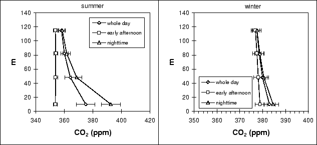
The long term, high precision concentration profiles give insight into the biochemical processes of the vegetation. High CO concentration accumulates close to the surface during nighttime in the growing season due to respiration, which is flushed out to the upper atmosphere during the morning transition period, when the nighttime inversion breaks up (Figure 3 in Haszpra, 1999a). This behaviour must appear in the measured vertical fluxes.

Figure shows the vertical profiles of carbon dioxide in winter and summer, in different time of the day. The summertime plot demonstrates the accumulation of CO during night, and the carbon uptake of the vegetation during daytime (CO concentration is lowest near the ground during daytime). The wintertime plot indicates the effect of accumulated carbon dioxide during the dormant season when respiration and soil CO efflux are the main determinatives of the carbon balance.

Figure: Vertical profiles of carbon dioxide mixing ratio in different seasons and in different time of the day at Hegyhátsál (error bar = ± /4) (The figure is taken from Haszpra, 1999a).

Since the objective of the present study is different from the above, no further details are presented here about the profiles, but simply refer to Haszpra (1999a).

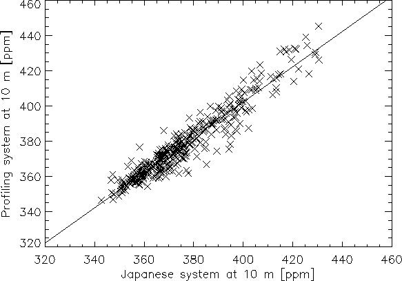
Figure shows the comparison of the CO concentration values measured by the profiling system at 10 m and the concentration values measured during the profile (or concentration) measuring periods of the Japanese system. The plot was produced using all available data from the Japanese system. The corresponding values were chosen such that the time difference between the time stamp of the Japanese data relative to the profiling data was less than 8 minutes. The Japanese data were averaged for 15 min intervals.

Figure: Comparison of the carbon dioxide concentration data in ppm measured by the Japanese system and the profiling system at 10 m. Number of samples: 377. The equation of the linear regression: , .

The plot was produced excluding some extreme differences, most probably caused by poor synchronization between the timer of the Japanese eddy covariance system and the internal clock of the profile data acquisition computer and by unusual instrument drift (as it was described in section , the Japanese system is calibrated for the whole day based on the calibration conducted short before midnight, while the profiling system is continuously accounted for instrument drift -- see section ).

The slope of the linear regression is 1.00154, and the intercept is 1.63, r=0.954. This indicates that the measured values are well correlated.