Three dimensional wind vector rotation is applied to the sonic anemometer data
following the method of Lee (1998). A general assumption for micrometeorological
measurements is the zero mean vertical wind speed. Generally, zero mean average
vertical wind speed is forced as part of the wind vector rotation routine (e.g.
McMillen, 1988). Lee proposes that this may be a good assumption very close
to the ground, but it is generally invalid at higher altitudes. The non-zero
mean vertical velocity is caused by local thermal circulations, topographically
modified flow, divergence in convective cell-like structures or synoptic scale
subsidence. The non-zero mean vertical wind speed transports heat, water vapor
and carbon dioxide across the plane of the actual measuring height, while this
transport is undetectable by the eddy covariance system, which is based on the
measurement of the fluctuating signals. Focusing on carbon dioxide, this transport
can be severe during nighttime, when carbon dioxide usually accumulating below
the inversion layer causing high vertical gradients of CO![]() near the
ground. As an example, a mean vertical velocity of 5 cm s
near the
ground. As an example, a mean vertical velocity of 5 cm s![]() at the
measuring height causes -100 W m
at the
measuring height causes -100 W m![]() equivalent energy flux for daytime
(or an uncertainty of about 20% of the observed net radiation).
equivalent energy flux for daytime
(or an uncertainty of about 20% of the observed net radiation).
As it is stated in Lee (1999), it is not appropriate to use the mean vertical wind speed measured by the sonic anemometer because of the low signal level, the possible sensor tilt and the aerodynamic shadow of the sensor or the tower. As it is proposed by Lee, the true mean vertical velocity can be approximated from the following equation:
Values of ![]() and
and ![]() are determined as functions of
are determined as functions of ![]() in 3
in 3![]() intervals using data from a previous complete run on the existing
database. Once the coefficients are determined, eq.
intervals using data from a previous complete run on the existing
database. Once the coefficients are determined, eq. ![]() can be used
to determine to calculate
can be used
to determine to calculate ![]() for each run. Horizontal rotation
is applied to the wind speed data such that
for each run. Horizontal rotation
is applied to the wind speed data such that ![]() is forced to
zero. Next, the coordinate system is rotated to ensure that the mean vertical
wind speed is equal to the one calculated using eq.
is forced to
zero. Next, the coordinate system is rotated to ensure that the mean vertical
wind speed is equal to the one calculated using eq. ![]() . The rotated
wind data is used to calculate turbulent fluxes and other statistics. The true
average vertical wind speed is finally stored for each hourly period. The
standard deviation of the lateral wind speed fluctuations (that is
. The rotated
wind data is used to calculate turbulent fluxes and other statistics. The true
average vertical wind speed is finally stored for each hourly period. The
standard deviation of the lateral wind speed fluctuations (that is ![]() after coordinate system rotation) together with the wind direction are also
stored in order to be able to calculate turbulent flux source areas in the future.
after coordinate system rotation) together with the wind direction are also
stored in order to be able to calculate turbulent flux source areas in the future.

|
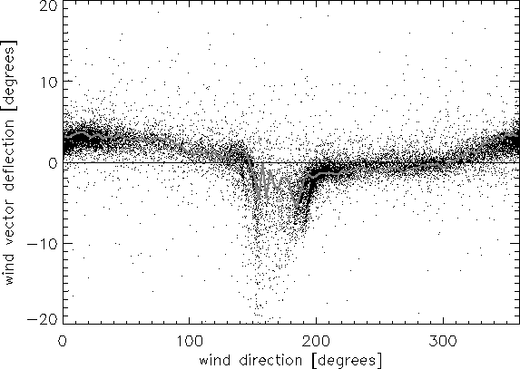
Figure ![]() shows the deflection of the average three dimensional
wind vector in the coordinate system defined by the instrument. The plot was
constructed using all available EC data. The solid grey line represents the
shows the deflection of the average three dimensional
wind vector in the coordinate system defined by the instrument. The plot was
constructed using all available EC data. The solid grey line represents the
![]() values (see eq.
values (see eq. ![]() ) for each 3
) for each 3![]() intervals calculated
using the least absolute deviation method. The effect of the tower body is clear
from the figure between wind direction 140
intervals calculated
using the least absolute deviation method. The effect of the tower body is clear
from the figure between wind direction 140![]() and 190
and 190![]() . There
is a sinusoidal behaviour outside this region which is caused by a slight tilt
of the instrument. This tilt is compensated using the above method proposed
by Lee (1998).
. There
is a sinusoidal behaviour outside this region which is caused by a slight tilt
of the instrument. This tilt is compensated using the above method proposed
by Lee (1998).
The application of the mean vertical velocity in the calculation of the net ecosystem exchange will be discussed later.