Direct comparison of surface fluxes computed from flux-profile relationships and by using eddy covariance, or from the two eddy covariance systems is complicated for non-homogeneous surfaces because the region of the surface (footprint and source area, Schmid, 1994, 1997) influencing each estimation may be different.
Horst (1999) shows that the source areas associated with fluxes measured by
application of similarity theory and the eddy covariance technique should be
approximately equal if the eddy covariance measurement is made at the effective
measuring height that is defined as the arithmetic mean of the elevations of
the highest and lowest profile measurements for stable stratification, or the
geometric mean for unstable stratification (Horst, 1999). In our case the effective
measuring height of the profile system is 28.6 m during unstable and 29 m during
stable conditions. Thus, the profile method and the two eddy covariance system
(82 m and 3 m) always represent different source areas in the mosaic-type terrain
(see fig. ![]() ). This may cause differences among the NEE values measued
by the three systems.
). This may cause differences among the NEE values measued
by the three systems.
Furthermore, fluxes determined by eddy covariance are expected to be reliable
even during slightly non-steady conditions, whereas the validity of the flux-profile
relationship is questionable for such conditions. Computational problems occur
during highly stable conditions due to the failure of convergence in the iterative
calculation method using the flux-profile relationship causing lack of flux
data during many nights. Intermittent turbulence at night also causes uncertainties.
The error correction routines outlined in section ![]() are
also a possible source of error due to the uncertainties in the temperature
reconstruction routine.
are
also a possible source of error due to the uncertainties in the temperature
reconstruction routine.
|
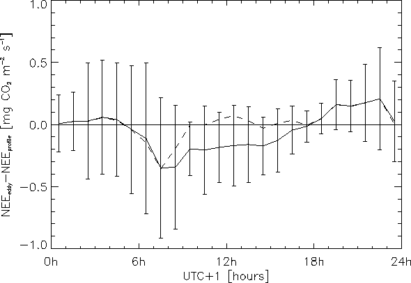
The net ecosystem exchange calculated from the first eddy covariance system
can be used to estimate the error term in the similarity theory calculation.
In our case, the mean daily cycle of the deviation of the profile fluxes from
NEE is calculated for each month using the data from all available years (Fig.
![]() , solid line). The data comparison shows that there is a systematic
underestimation of NEE calculated from the profile method during daytime, and
a smaller systematic overestimation during nighttime. There is an emphasized
underestimation during the morning transition period. Construction of a new,
site specific similarity function for CO
, solid line). The data comparison shows that there is a systematic
underestimation of NEE calculated from the profile method during daytime, and
a smaller systematic overestimation during nighttime. There is an emphasized
underestimation during the morning transition period. Construction of a new,
site specific similarity function for CO![]() based on the existing NEE
data, following the method of e.g., Högström (1988), gave better results,
but the problem of the morning transition period was not solved (Fig.
based on the existing NEE
data, following the method of e.g., Högström (1988), gave better results,
but the problem of the morning transition period was not solved (Fig. ![]() ,
dashed line). This problem can be eliminated if the calculated monthly average
daily deviations are simply added to the daily profile CO
,
dashed line). This problem can be eliminated if the calculated monthly average
daily deviations are simply added to the daily profile CO![]() flux data
calculated from the similarity theory.
flux data
calculated from the similarity theory.
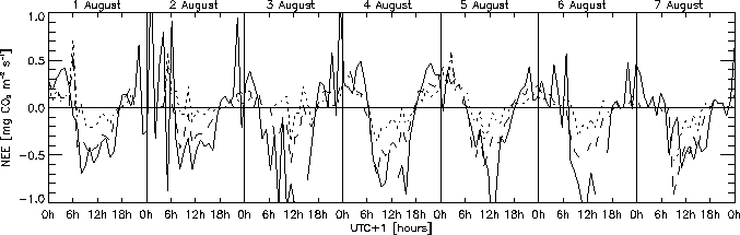
Figure ![]() compares the NEE calculated from the profile data by
means of the surface layer similarity theory and from the direct flux measurements
by means of the eddy covariance technique at 82 m for a continuous 7 day period
between 1 August and 7 August, 1998. During this period daily mean temperature
ranged between 19
compares the NEE calculated from the profile data by
means of the surface layer similarity theory and from the direct flux measurements
by means of the eddy covariance technique at 82 m for a continuous 7 day period
between 1 August and 7 August, 1998. During this period daily mean temperature
ranged between 19![]() C and 26
C and 26![]() C, and there was no precipitation.
A cold frontal overpass occured between the 3rd and 5th of August, causing partial
cloudiness during the 4th and 5th of August.
C, and there was no precipitation.
A cold frontal overpass occured between the 3rd and 5th of August, causing partial
cloudiness during the 4th and 5th of August.
The figure shows the raw, unmodified profile fluxes (dotted line) vs. NEE (solid line), and the modified similarity fluxes (dashed line). The matching of the data is significantly improved with the method applied.
|
In summary, flux estimates based solely on the theoretical flux-profile relationships from similarity theory do not provide accurate, long-term carbon budget estimates due to both random and systematic errors, and site specific factors. Since selective-systematic errors can change even the sign of the long-term net carbon dioxide budget of a region (Moncrieff et al., 1996), these errors can cause significant bias in the overall regional net source/sink estimation. In spite of this weaknesses of the profile flux dataset, it is useful for filling the data gaps that inevitably occur during long-term eddy covariance measurements. The application of the ``tweaked'' profile fluxes in the estimation of the net carbon balance of the region is described below.
Comparison of the eddy covariance based NEE measured at 3 m and 82 m is not
straightforward. The 82 m NEE is a measure of the overall behaviour of the surrounding
forest patches, cultivated areas, vineyards, settlements, etc. The flux source
area is clearly changing day-by-day, and during each specific day, so there
is no reason to tie the results to any specific biome type (C![]() or
C
or
C![]() crops, trees, etc.). In contrast, the 3 m system has a very limited
source area (the surrounding 300 m radius circle according to the micrometeorological
rule-of-thumb (Businger, 1986)). Thus, the area ``sensed'' by the instruments
is more definite.
crops, trees, etc.). In contrast, the 3 m system has a very limited
source area (the surrounding 300 m radius circle according to the micrometeorological
rule-of-thumb (Businger, 1986)). Thus, the area ``sensed'' by the instruments
is more definite.
Keeping all the above in mind, we may compare the NEE measured by the two, independent system.
|
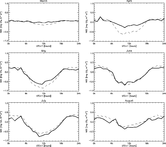
Figure ![]() shows a comparison of the calculated monthly mean
daily NEE cycles measured by the 82 m system and the 3 m system for six months
in 1999. The monthly averages are calculated directly from the measured NEE
data, not utilizing any gap filling routine for missing data.
shows a comparison of the calculated monthly mean
daily NEE cycles measured by the 82 m system and the 3 m system for six months
in 1999. The monthly averages are calculated directly from the measured NEE
data, not utilizing any gap filling routine for missing data.
The figure shows that the vegetation around the TV transmitter tower (mainly
grassland) starts to act as a sink of CO![]() earlier compared to the
average behaviour of the vegetation in a larger scale (arable land and forest
patches). In March 1999 the 82 m system detected a net loss of CO
earlier compared to the
average behaviour of the vegetation in a larger scale (arable land and forest
patches). In March 1999 the 82 m system detected a net loss of CO![]() from the biosphere to the atmosphere, while the small scale system detected
a net gain of CO
from the biosphere to the atmosphere, while the small scale system detected
a net gain of CO![]() . This may be caused by the early activity of the
grassland around the tower site. The nighttime respiration rates are very similar
at this part of the year. During April, the monthly net budget changed sign
as it is measured by the 82 m system, but the daytime photosynthetic rates are
still lower here compared to the 3 m system. This difference persists during
May, when the maximum value of the 3 m NEE is about 0.85 mg CO
. This may be caused by the early activity of the
grassland around the tower site. The nighttime respiration rates are very similar
at this part of the year. During April, the monthly net budget changed sign
as it is measured by the 82 m system, but the daytime photosynthetic rates are
still lower here compared to the 3 m system. This difference persists during
May, when the maximum value of the 3 m NEE is about 0.85 mg CO![]() m
m![]() s
s![]() (19.3
(19.3 ![]() mol m
mol m![]() s
s![]() ) but only 0.7 mg CO
) but only 0.7 mg CO![]() m
m![]() s
s![]() (15.9
(15.9 ![]() mol m
mol m![]() s
s![]() ) for the 82 m system. The nighttime
respiration measured by the 3 m system starts to exceed the 82 m respiration.
In June, the daytime NEE are approximately the same for the two scale reaching
almost 0.7 mg CO
) for the 82 m system. The nighttime
respiration measured by the 3 m system starts to exceed the 82 m respiration.
In June, the daytime NEE are approximately the same for the two scale reaching
almost 0.7 mg CO![]() m
m![]() s
s![]() (15.9
(15.9 ![]() mol m
mol m![]() s
s![]() )
around noon. This is lower than the 3 m average value in May. The 3 m respiratory
rates are higher that the 82 m rates. As we will see it later, this difference
restricts the carbon balance of the tower's surroundings. Daytime 82 m NEE exceeds
the 3 m value in July, while the respiration remains higher for 3 m. The large
scale average NEE reaches 0.8 mg CO
)
around noon. This is lower than the 3 m average value in May. The 3 m respiratory
rates are higher that the 82 m rates. As we will see it later, this difference
restricts the carbon balance of the tower's surroundings. Daytime 82 m NEE exceeds
the 3 m value in July, while the respiration remains higher for 3 m. The large
scale average NEE reaches 0.8 mg CO![]() m
m![]() s
s![]() (18.2
(18.2 ![]() mol m
mol m![]() s
s![]() )
during daytime. August exhibits similar behaviour as June, with a considerably
lower daytime carbon uptake rate (less than 0.4 mg CO
)
during daytime. August exhibits similar behaviour as June, with a considerably
lower daytime carbon uptake rate (less than 0.4 mg CO![]() m
m![]() s
s![]() (9.1
(9.1 ![]() mol m
mol m![]() s
s![]() )). This lower value is caused
by changes in the environmental conditions (see later).
)). This lower value is caused
by changes in the environmental conditions (see later).
The comparison demonstrates the effect of the different flux source areas on the ensemble monthly cycles of NEE as measured by the two measuring system.
Figure ![]() shows the comparison of a weekly NEE time series
measured by the 82 m and the 3 m system between 12 June and 18 June, 1999. During
this period daily mean temperature ranged between 16
shows the comparison of a weekly NEE time series
measured by the 82 m and the 3 m system between 12 June and 18 June, 1999. During
this period daily mean temperature ranged between 16![]() C and 18
C and 18![]() C.
1.2 mm precipitation fell in 15 June and 6.9 mm during 17 June. There was no
frontal activity except during 12 June, but the sky was frequently covered by
clouds during the whole period.
C.
1.2 mm precipitation fell in 15 June and 6.9 mm during 17 June. There was no
frontal activity except during 12 June, but the sky was frequently covered by
clouds during the whole period.
The daily courses of NEE are very similar in many cases in spite of the different source areas, but there are some differences that are attributed to the different scale (e.g. during 14 June).
|
NEE peaks at about noon for both system and can exceed 1.4 mg CO![]() m
m![]() s
s![]() (31.8
(31.8 ![]() mol m
mol m![]() s
s![]() ) for the 82 m system (the absolute
maximum for the whole measurement is around 1.5 mg CO
) for the 82 m system (the absolute
maximum for the whole measurement is around 1.5 mg CO![]() m
m![]() s
s![]() (34.1
(34.1 ![]() mol m
mol m![]() s
s![]() )), and about 1.2 mg CO
)), and about 1.2 mg CO![]() m
m![]() s
s![]() (27.3
(27.3 ![]() mol m
mol m![]() s
s![]() ) for the 3 m system. During
May, when NEE at 3 m is the largest, its maximum reaches the maximum of NEE
at 82 m. The nighttime respiration at 3 m is somewhat larger than for 82 m as
it is expexted from the monthly averages.
) for the 3 m system. During
May, when NEE at 3 m is the largest, its maximum reaches the maximum of NEE
at 82 m. The nighttime respiration at 3 m is somewhat larger than for 82 m as
it is expexted from the monthly averages.
Other feature of the plot is a phenomenon that is experienced several times
during the growing season: during nighttime the vegetation might appear to be
a sink for a few hourly periods, and these periods are connected with very high,
rapidly changing outgoing NEE in the neighbouring intervals (between 0-6 h in
14 June). This might be caused by intermittent turbulent processes that flushes
the accumulated CO![]() out of lower air layer. The sink behaviour during
nighttime is ecologically incorrect, but can be explained by the rapid change
of the storage: if a flush-out event occurs, the CO
out of lower air layer. The sink behaviour during
nighttime is ecologically incorrect, but can be explained by the rapid change
of the storage: if a flush-out event occurs, the CO![]() storage of the
air layer below 82 m indicates CO
storage of the
air layer below 82 m indicates CO![]() uptake of the vegetation. If the
change of the storage term is not compensated by a strong apparent eddy flux
at 82 m, or if this flux is detected later (which means that it reaches the
82 m level later), NEE indicates CO
uptake of the vegetation. If the
change of the storage term is not compensated by a strong apparent eddy flux
at 82 m, or if this flux is detected later (which means that it reaches the
82 m level later), NEE indicates CO![]() uptake by the vegetation. If
this is the case, a peak is expected later during the night, which is of course
caused by the restored normal storage change and the previously flushed CO
uptake by the vegetation. If
this is the case, a peak is expected later during the night, which is of course
caused by the restored normal storage change and the previously flushed CO![]() .
These peaks are visible in the figure. It should be noted, that this phenomena
does not cause bias in the net daily CO
.
These peaks are visible in the figure. It should be noted, that this phenomena
does not cause bias in the net daily CO![]() ecosystem exchange since
all neccesary terms are measured, although not in the same time (i.e. the peaks
compensate each other). Horizontal advection might also play important role
in the above phenomena (Yi et al., 2000).
ecosystem exchange since
all neccesary terms are measured, although not in the same time (i.e. the peaks
compensate each other). Horizontal advection might also play important role
in the above phenomena (Yi et al., 2000).
All of the above raise the need for a flux footprint/source area model to investigate the area of representativeness for the EC-based systems. Due to the complexity of the problem (Schmid, 1994, 1997; Horst, 1994, 1999), there is no appropriate model available for practical purpose. The mini-FSAM model of Schmid (1994) is a promising, tiny, easy to use flux source area model, but as it is admitted by the same author (Schmid, 1997), it became clear that the earlier calculations had contained mistakes, thus the model should not be used for source area calculations in any way. A possible future aim of the current project is the development of a model which can be used in practice to determine the area of representativeness for the measurements as a routine task.