|
Based on the long term measurement data, we can investigate the response of the measured NEE to the environmental factors. The main variables controlling the behaviour of the vegetation is the incoming photosynthetically active photon flux density (PPFD), temperature, soil mositure and vapor pressure deficit (VPD, defined as the difference between the saturated water vapor pressure and the actual water vapor pressure at a given temperature in the atmosphere).
PPFD is the most immediate environmental control on photosynthesis (Malhi et al., 1999). The major influence of temperature on net carbon balance is through its effects on rates of both autotrophic and heterotrophic respirations (Malhi et al., 1999). Since we can not distinguish between these two types, we may only describe the net effect of respiration. Vapor pressure deficit controls stomatal closure, thus it has a direct effect on the rate of photosynthesis. High VPD causes stomatal closure, decreasing photosynthesis (Anthoni et al., 1999). Lack of soil moisture also reduces carbon uptake by causing stomatal closure, but also affects soil carbon and nutrient release by restricting microbial decomposition (Malhi et al., 1999).
PPFD, VPD and air temperature are currently measured by our system. Soil moisture measurement will be installed in the near future at Hegyhátsál.

|
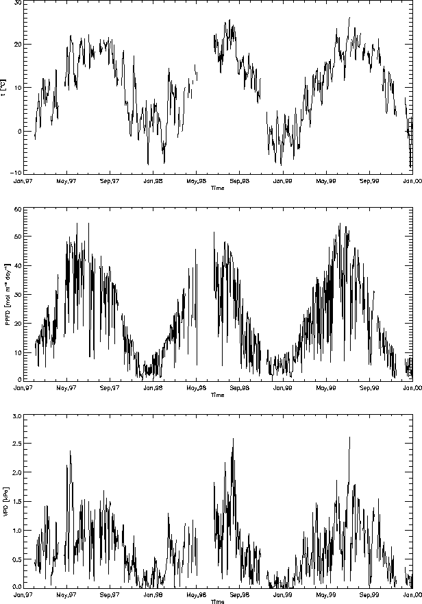
Figure ![]() shows the temporal course of the daily aggregated environmental
variables controlling the carbon budget of the vegetation for 1997, 1998 and
1999 (i.e. for the whole 82 m EC measurement period, so far3.1).
shows the temporal course of the daily aggregated environmental
variables controlling the carbon budget of the vegetation for 1997, 1998 and
1999 (i.e. for the whole 82 m EC measurement period, so far3.1).
Based on the PPFD and NEE time series, it is possible to construct the light response function of NEE for the different months during the growing season. This can be used for modelling purposes.
Figure ![]() shows the NEE-PPFD function for August, 1997-1999.
Data was measured between 8 h and 19 h UTC+1. Number of samples = 788. NEE was
classified by the measured VPD. The figure shows that on average, higher VPD
causes slight decrease (in absolute meaning) of NEE, as it is expected from
the theory. The fitted equation is a Michaelis-Menten type rectangular hyperbola
(Valentini et al., 1996; Markkanen et al., 2001). The NEE-PPFD function has
the following form (solid line in figure
shows the NEE-PPFD function for August, 1997-1999.
Data was measured between 8 h and 19 h UTC+1. Number of samples = 788. NEE was
classified by the measured VPD. The figure shows that on average, higher VPD
causes slight decrease (in absolute meaning) of NEE, as it is expected from
the theory. The fitted equation is a Michaelis-Menten type rectangular hyperbola
(Valentini et al., 1996; Markkanen et al., 2001). The NEE-PPFD function has
the following form (solid line in figure ![]() ):
):

|
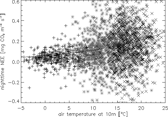
Figure ![]() shows the NEE-air temperature function (air temperature
measured at 10 m is used) during nighttime for March-August, 1997-1999. Number
of samples used for fitting = 3356 (includes data from March-October, 1997-1999;
September-October data is not plotted but used for fitting). Nighttime period
before day of year (DOY) 100 and after DOY 260 is defined as the period between
18 h and 5 h UTC+1, and the period from 20 h till 3 h between DOY 100 and DOY
260. The fitted curve has the following form:
shows the NEE-air temperature function (air temperature
measured at 10 m is used) during nighttime for March-August, 1997-1999. Number
of samples used for fitting = 3356 (includes data from March-October, 1997-1999;
September-October data is not plotted but used for fitting). Nighttime period
before day of year (DOY) 100 and after DOY 260 is defined as the period between
18 h and 5 h UTC+1, and the period from 20 h till 3 h between DOY 100 and DOY
260. The fitted curve has the following form:
Outside the March-October period, another NEE-![]() function is constructed
using both daytime and nighttime data using data from all available years. The
coefficients of the fitted curve are
function is constructed
using both daytime and nighttime data using data from all available years. The
coefficients of the fitted curve are ![]() and
and ![]() (data
not shown). This curve shows good agreement with the previous one in the -5 - 0
(data
not shown). This curve shows good agreement with the previous one in the -5 - 0![]() C
interval. This curve is supposed to be used for NEE modelling purposes both
for daytime and nighttime in this period as a function of air temperature.
C
interval. This curve is supposed to be used for NEE modelling purposes both
for daytime and nighttime in this period as a function of air temperature.
The same procedure is performed for the Japanese system. Air temperature measured
by the Kaijo-Denki anemometer/thermometer at 3 m was used to determine the NEE-![]() relationship during nighttime. PPFD measured by the profile system was used
to fit the NEE-PPFD curves in the same way as it is done in the case of the
82 m system.
relationship during nighttime. PPFD measured by the profile system was used
to fit the NEE-PPFD curves in the same way as it is done in the case of the
82 m system.
Coefficients of the light response curve are presented in table ![]() for the growing period of 1999 (except October, when no PPFD data was available).
for the growing period of 1999 (except October, when no PPFD data was available).
|
During the vegetative period, one NEE-![]() curve is constructed similarly
to the 82 m system. Since air temperature at 3 m is measured by the system,
the ensemble temperature response curve is estimated from all available data
from 1999 and 2000. The coefficients of this ensemble curve are
curve is constructed similarly
to the 82 m system. Since air temperature at 3 m is measured by the system,
the ensemble temperature response curve is estimated from all available data
from 1999 and 2000. The coefficients of this ensemble curve are ![]() and
and ![]() , to be used with eq.
, to be used with eq. ![]() for months between March
and October. The Q
for months between March
and October. The Q![]() coefficient is 2.23 here. This is higher than
that estimated for 82 m for the same period mainly caused by the higher respiration
rates of the vegetation (see fig.
coefficient is 2.23 here. This is higher than
that estimated for 82 m for the same period mainly caused by the higher respiration
rates of the vegetation (see fig. ![]() ) that is sensed by the
3 m system (source area, see section
) that is sensed by the
3 m system (source area, see section ![]() ) during nighttime.
) during nighttime.
For months between November and February, the exponential function defined by
![]() and
and ![]() should be used both for daytime and nighttime.
should be used both for daytime and nighttime.